Creating your Application
This guide introduces you on how to write a simple application using the PACO components. It is divided into two sections based on the components you wish to use. These two components can also be combined to create a binary in which you could use both of them.
Alright! Let’s get started!
1. Decide on the Approximate Component to Use
2. LUT Guide
The Lookup Table (LUT) is a functional unit residing in the CPU pipeline and can be imagined as a software lookup table on crack. It’s main purpose is to approximate any derivable function. To visualize it, let’s take a look at the graph of a function:
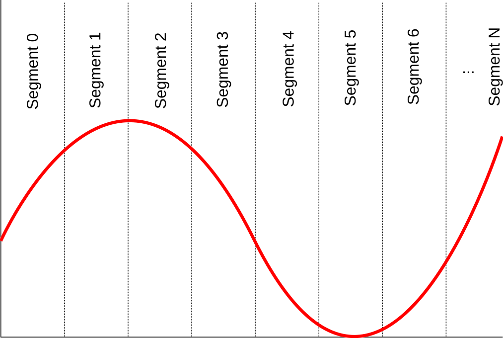
In order to approximate this function, it needs to be divided into several intervals, here called segments. The above image shows a linear distribution of segments. Using the PACO tools, you could also choose from other distributions such as a logarithmic distribution (see Developers Guide). These primary segments can also be further divided into secondary segments giving you fine grained control over the function you wish to approximate.
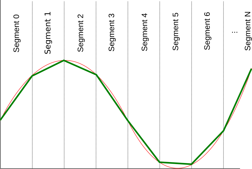
For each segment we can now interpolate the function. The picture below shows a linear interpolation for every segment. The interpolated line of each segment can then be stored as integer values m, b in our LUT. With the formula y = m * x + b we can describe the line again.
For more information on the LUT please read the Design Document
A suitable application for the LUT is the Gamma correction image filter since it uses an expensive exponentiation which can be approximated. Thus we use it as an example for this tutorial.
The complete code for this example, including a Makefile can be found here
2.1 Select your function to be approximated
Firstly we have to implement our function in normal C code. You can see our implementation below:
#include <math.h>

long image[IMG_WIDTH * IMG_HEIGHT];
long result_image[IMG_WIDTH * IMG_HEIGHT];

/* This is the implementation of our gamma correction */
long gamma(long a)
{
  double v;
  int r;
  v=(double)a/(double)(1uL<<24);
  v= 1.0 * pow(v,0.25);
  if (v>1) v=1; else if (v<0) v=0;
  r=(int)(v*(double)(1uL<<24));
  return r;
}

int main()
{
    int i;
    long inp;

    for(i = 0; i < IMG_WIDTH * IMG_HEIGHT; i++) {
        /* since we use greyscale images, we shift
           the data into the red channel */
        inp = image[i] << 16;
        result_image[i] = gamma(inp);
    }
}
Now that we have our function, we need to tell the compiler to use the LUT for this implementation. We also have to decide on how to divide the function into segments and the range on the x-axis on which it is divided. This is done using annotation, which will be covered in the next section.
2.2 Annotate your function for approximation
Firstly we need to tell the compiler that our function gamma should be approximated. We do this by adding the approx decorator to the function. Then, we need to indicate that we want to use the LUT for approximating the function. This can be done by adding the keyword strategy=”lut” to the decorator.
long approx(strategy="lut") gamma(long a)
{
/* ... */
}
Now that the compiler knows that this function should be approximated using the LUT, we can provide hints on how the approximation should be performed. We do this by adding several key/value pairs to the approx decorator. The code snippet below shows some of the options:
long approx(strategy="lut" numPrimarySegments="6" bound="(0,16777215)" segements="uniform" approximation="linear") gamma(long a)
{
/* ... */
}
This is what the key/value pairs we used above mean:
- numPrimarySegments indicates the number of primary segments used for approximation. Since we don’t subdivide our segements into subsegments, this is also the total number of segments.
- bound indicates the range of the input values of our function. It is given as a list of intervals (min, max), (min, max),.. . For example let us consider an image. There are 3 colors with 8 bits per pixel, which leads to a maximum value of (2⁸)³ = 16777216 and a minimum value of 0. Therefore, the bound can be provided as bound=”(0,16777215)” as in the example above.
- segments indicates how the segments are distributed. In this case, it is uniformly distributed, as shown in the pictures in Section 2.
- approximation indicates how the function is approximated within each segment. “Linear” in this case means that it is approximated using a line, as can be seen in the picture of section 2.
For more information on other possible key/values please read Annotate Code.
2.3 Compile your program
The basic steps to compile you program are (for more details, refer to User Guide):
- Compile you program using Clang. This will yield an llvm-ir file of your code and an input file to the LUT-compiler.
- Use llc to convert the LLVM-IR file into an assembly file.
- Invoke the lut-compiler on the input file to generate a configuration for the LUT.
- Use the lut-startup script with the configuration to create a startup code that loads the configuration.
- Link everything together into a binary.
Now you should have a binary ready to be run on an FPGA.
2.4 Run your program on the FPGA
For instructions on how you can run your program on the FPGA please take a look here.
3. Approximate ALU Guide
The PACO Approximate ALU approximates by neglecting some of the least significant bits of an operation such as add, sub, or mul. This effect can be accomplished only in certain applications. Since its not possible to automatically discern the variables that supports the approximation operation, you, as the programmer, need to annotate the variables as approximate. The next section will show you how to do just that.
For this example we will use a Gaussian blur image filter with the following kernel matrix:
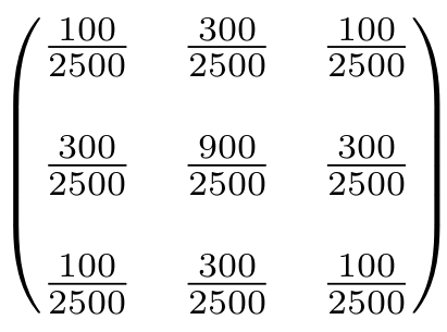
The complete code for this example, including a Makefile can be found here.
3.1 Select the variables which can be imprecise
Let’s say, we have the following program snippet implementing this filter:
long image[IMG_WIDTH * IMG_HEIGHT];
long result_image[IMG_WIDTH * IMG_HEIGHT];
long kernel[9] = {100, 300, 100,
                  300, 900, 300,
                  100, 300, 100};
void gauss()
{
    long image_data;
    long kernel_data;
    long intermediate_data;
    long result;

    for (x = 1; x < IMG_WIDTH - 1; x++) {
        for (y = 1; y < IMG_HEIGHT - 1; y++) {
            image_data = image[(y - 1) * IMG_WIDTH + (x - 1)];
            kernel_data = kernel[0];
            intermediate_data = image_data * kernel_data;
            result = result + intermediate_data;

            image_data = image[(y - 1) * IMG_WIDTH + (x      )];
            kernel_data = kernel[1];
            intermediate_data = image_data * kernel_data;
            result = result + intermediate_data;

            /* .... */
            result /= 2500;
            result_image[y * IMG_WIDTH + x] = result;
        }
    }
}
The variables image_data, intermediate_data, and result would be suitable candidates for approximation because these contain the image data intended to be seen by humans. Therefore, approximating them would be ideal since the human eye cannot perceive minor errors.
The next section explains on how to mark these variables for approximation.
3.2 Annotate variables for approximation
We annotate a variable with approximate decorators as follows:
/* ... */
void gauss()
{
    long approx(neglect_amount=2 inject=1)image_data;
    long kernel_data;
    long approx(neglect_amount=2 inject=1 relax=1)intermediate_data;
    long approx(neglect_amount=2, inject=1 relax=1)result;
}
An approx decorator can have key/value pairs, which further describe how a variable can be approximated. For example: neglect_amount=2 indicates that the compiler has to neglect the least 2 significant bits during an operation. If we take a look at the following code snippet from the gauss function,
long approx(neglect_amount=2 inject=1 relax=1)intermediate_data;
long approx(neglect_amount=2, inject=1 relax=1)result;
/* since "intermediate_data" and "result" both can be approximated the compiler would emit a add.approx instruction here. */
result = result + intermediate_data;
we can notice that if an operation uses two variables with approx decorators, an approximate operation will be emitted. In this particular case, it would be an add.approx or an approximate addition operation.
In the next section, you will learn how to compile your program and how this particular code snippet would be translated to assembly. If you want to read more regarding annotations, take a look here
3.3 Compile your program
Compiling your program takes nothing more than invoking Clang. The details on compiling Clang/llvm and the parameters to use for example, using the correct ISA backend, please refer to the User Guide
However for now lets see how our compiler would translate the code snippet from above by running objdump on int
$ riscv64-unknown-elf-objdump -S main.elf

  ...

  0000000000000184 <.Ltmp41>:
            immediate  = image_data * kernel_data;
  184:   fca3a38b                mul.approx      t2,t2,a0,0x3f

  0000000000000188 <.Ltmp42>:
            result = result + immediate;
  188:   f873030b                add.approx      t1,t1,t2,0x3e

  ...
Well, the compiler emitted the add.approx instruction. The last parameter of this instruction is the amount of bits to neglect.
Congratulations! You have successfully created your first approximate program using PACO. Now onto how it performs on the FPGA.
3.4 Run your program on the FPGA
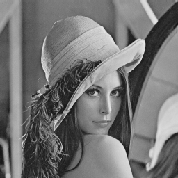
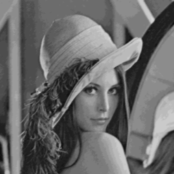
For instructions on how you can run your program on the FPGA please take a look here. For now, let us compare how approximation affects the image. The default test image that we used for our graphical application is Lenna as can be seen below in grey-scale.
Our approximated program with a neglect_amount of 4, on applying the gaussian filter produces this image:
Let’s compare it against our program that applies the gaussian filter without any approximate decorators:
